Gaussian Integral Notes (Scalar Field Theory Part 1)

This is a set of notes moving towards the simplest statistical or quantum field theory of all: the free scalar field. In part 1, I cover some of the gory details about the multivariate Gaussian integral and multivariate Gaussian probability distribution. I don’t specialize to a specific form of covariance matrix, and I try to include as many neat facts as I know. This is the reference I wish I read or wrote way back in 2017 when I first learned all this stuff.

If you’re studying quantum field theory then a solid 80% of this material should be second nature to you. Stuff like Schur complements, the affine conditional section, or finding $Z(0)$ for any partition function, are less important.

Stand-outs here include: “conditioning on constant mass introduces negative correlations”, a formula for a Gaussian conditioned on a system of independent affine-linear constraints, and a mention of the equipartition theorem. It’s especially fun to apply weird constraints to samples of Gaussian processes:

This is discussed in the way I’ve learned about it in my physics coursework, so if you find yourself saying “this is the most stupid way to discuss this basic probability fact that I’ve ever seen,” you might be right!

Wick’s theorem is not discussed in as much detail as it deserves, and I do not apply it to perturbation theory here.

Directory

• 1. The Partition Function
• 2. Expectation Values
  • Bringing the Expectation Inside the Exponent
  • Ward and Schwinger-Dyson
• 3. Marginalizing and Conditioning to Zero
  • Marginalizing
  • Conditioning
• 4. Conditioning on an Affine-Linear Constraint
  • Conditioned Expectation Values via Integration
  • Conditioned Expectation Values via Projection
  • An Example of Conditioning: Fixed Total Mass
• 5. As an Integral over Shells
• 6. Sampling from a Multivariate Gaussian
  • Sampling given the Covariance Matrix
  • Sampling given the Hessian
  • One-Dimensional Gaussian Field Examples
• Appendix: Extra derivations and Practice Problems
  • Schur Complements
  • Fresnel Integral Derivation

1. The Partition Function

For a positive definite and symmetric linear operator $A$ in $d$ dimensions,

Furthermore, we often want a vector J called a source term, where we write:

The matrix $A$ is the inverse covariance matrix (proved later). It is also called the Hessian matrix because it often arises in physical settings from a Taylor expansion.

2. Expectation Values

Suppose we care about expectation values of the field value $x_i$ evaluated at some source term $J=h.$ We find the mean $\mu:$

For the two point correlation function, we find

where $\Sigma=A^{-1}.$ A very neat trick is that if we then want to calculate the connected correlation function

we can simply compute $\frac{\partial}{\partial J_ i}\frac{\partial}{\partial J _ j} \log(Z(J))\big| _ {J=h},$ giving the covariance matrix $\Sigma:$

So our important result is that any distribution proportional to $\exp\left(-x^T A x/2 + h^T x\right)$ has covariance and mean given by:

In general, we may write any correlation function in terms of Wick’s theorem. We usually only care about the case where $\mu=0,$ where:

For example,

If we’re feeling crazy we can let the mean be nonzero. The sum is taken over all partial Wick pairings on $n$ points:

Bringing the Expectation Inside the Exponent

For a distribution $P(x)\propto \exp(-\frac{1}{2}x^T A x+h^T x),$ we of course have

If we take $h=0,$ this gives the expression (with the repeated index summation convention)

which can surprise you if you’re suddenly wondering how the expectation value wound up inside the exponent!

This is a corollary of the cumulant expansion which holds for any reasonable probability distribution:

where $\kappa_n$ is the $n$th cumulant of the random variable $y$ (mean, variance, and so on). For a random variable which depends linearly on the Gaussian coordinates, such as $y=J^t x,$ we have $\kappa_n(y)=0$ for all $n\ge 3,$ so this ends up being particularly simple.

Note that if $y$ is not a Gaussian random variable then the situation is much more complicated and $\kappa_n(y)$ will not truncate, nor be simple to calculate! This complexity includes the situation where $y$ depends in a nonlinear way on the Gaussian random variables $x.$

Ward and Schwinger-Dyson

The Schwinger-Dyson equation can be derived from the fact that, for a reasonably well-behaved function $F:$

Expand and multiply through by $\Sigma$ to find (repeated index summation convention):

This can be used to derive Wick’s theorem.

Another identity is the Ward identity. The Ward identity won’t blow us away here, it’s equivalent to the Schwinger-Dyson equation for our case, but it’s conceptually different. Suppose we care about $\langle F\rangle,$ and we redefine our fields $y= x+\varepsilon v(x).$ The Jacobian transforms as $\mathrm{d}^d y=(\det \partial y/\partial x)\mathrm{d}^d x$. $\partial y_i/\partial x_j=\delta_{ij} +\varepsilon \partial v_i/\partial x_j,$ and to first order $\det(I+\varepsilon M)=1+\varepsilon \operatorname{tr} M.$ I adopt the repeated index summation convention and expand the whole thing in gory detail:

The term proportional to epsilon must vanish, so for any reasonable vector field $v$ and observable $F,$

Why doesn’t this blow us away? Because it can be derived by simply applying the Schwinger-Dyson equation to $F’=v_i F.$ But the interpretation is important, and in quantum field theory it’s also important when $v_i$ is a symmetry of the system. There the action $S=\frac{1}{2}x^T A x-h^T x$ and for a symmetry we may have $\partial_i v_i=0$ and $v_i \partial_i S=0.$ Our Ward identity is then $\langle v_i \partial_i F\rangle =0.$

3. Marginalizing and Conditioning to Zero

As a reminder, if we have a continuous joint probability distribution $P(x,y)$, marginalizing the variable $y$ gives a distribution

while conditioning on the variable $y$ gives

Marginalizing

For marginalizing on a variable $x_i$ in a multivariate Gaussian, performing the integral $\textrm{d}x_i$ explicitly is a bit tedious (though it’s just completing the square in the exponent). The key is that marginalizing doesn’t change expectation values. So $\Sigma_{jk}$ is unchanged, except at row and column $i.$ We conclude that marginalizing deletes rows and columns of the covariance matrix.

The Hessian view of marginalization is a bit more difficult. Say we split our Hessian up into blocks, and we want to integrate out the variables $\mathrm{d}^3 v$.

Upon performing the Gaussian integrals (completing the square in the exponent), we find a new marginalized Hessian and source:

$A_{\mathrm{marg}}$ is called the Schur complement of the block $A_{vv}$ in $A.$ The Schur complement is discussed in the appendix as a problem set. I find it a bit funny that the expression for $h_{\mathrm{marg}}$ takes a bit of work, even though the mean $\mu_u$ is unchanged!

Conditioning

If a multivariate Gaussian is given in terms of the Hessian, then conditioning on $x_i=0$ for some $i$ is trivial, because this simply deletes the relevant rows and columns from the Hessian.

How does the covariance matrix change in terms of the Hessian? It’s the Schur complement again! Suppose we condition on a set of variables $v=0,$ where:

Then conditioning gives:

4. Conditioning on an Affine-Linear Constraint.

Conditioning on a general linear constraint $a\cdot x=b$ shifts the mean and reduces the rank of the covariance matrix by one, so the Hessian and covariance matrices are no longer cleanly inverses of each other. Working through the formulas for this now will help us later in finding an algorithm to sample from a conditioned Gaussian. The PDF of a conditioned Gaussian is given by

If we find $\langle x_i\rangle$ and $\langle x_i x_j\rangle_c,$ we know everything there is to know about the constrained distribution. We’ll do this two ways, first by integration, and second by thinking about how to project the vector $x$ into the relevant hyperplane.

Conditioned Expectation Values via Integration

The trick here is to write $\delta(x)=\int \frac{dk}{2\pi}e^{ikx},$ then do the integral $\textrm{d}^d x,$ then do the integral $\textrm{d}k.$ It is useful to shift the integral to $x’=x-\mu$ and $c=b-a^T \mu.$ Also, let $Z_0(J)$ be the value of the partition function without the delta function prefactor. We find…

Completing the square in the exponent gives

Completing the integral $\mathrm{d}^dx$ just gives a factor of $Z_0(0)$, and we can take the factor of $\exp(J^T\mu+\frac{1}{2}J^T A^{-1}J)$ as well to get $Z_0(J)$. Let’s also stop writing $A^{-1}$ and start writing $\Sigma$ instead. Then:

by factoring out all J dependence in the exponent and completing the square. We can read off that

and

Conditioned Expectation Values via Projection

If we don’t like evaluating integrals, there is a more procedural way to think about finding the conditioned expectation value. The idea is to sample $x$ from the full Gaussian (so $x\sim \mathcal{N}(\mu,\Sigma)$) and then do an affine projection to the plane $a^Tx=b.$ We call this operator $\operatorname{Proj},$ and we consider only projections with $\operatorname{Proj}(x)=x$ for points which satisfy $a^T x=b.$ Then we naturally have an equality of probability distributions $P(\operatorname{Proj}(x)|a^Tx=b)=P(x|a^Tx=b).$ We can go one step further: if this projection has the magical property that

then the distribution of the projection of $x$ is exactly the conditioned distribution we’re searching for. A sufficient condition for this is if $a^Tx$ and $\operatorname{Proj}(x)$ are statistically independent. Because these are both Gaussian random variables, they are independent if and only if their covariance is zero. So we have our proof strategy: select a $\operatorname{Proj},$ then find the covariance of $a^Tx$ and $\operatorname{Proj}(x)_i$, and if this covariance is zero our proof is done.

There are many possible projections to the plane, one choice would be to look at the orthogonal projection under the Euclidean metric, but we would find this doesn’t have the independence properties we need. After some trial and error we find that the appropriate metric arises from minimizing the distance function $\frac{1}{2} x^T \Sigma^{-1} x.$ The projection of some point $y$ to the plane given by this metric is given by the result of the Lagrange minimization problem:

This gives the following affine projection:

I find it convenient to write our affine projection $\operatorname{Proj}(x)$ in terms of a base point $x_0$ and a linear operator $\hat{P},$ with $\operatorname{Proj}(x)=x_0+\hat{P}(x-x_0).$ A convenient choice of $x_0$ is the projection of $\mu:$

To find the linear part of the projection, it’s best to read it off or intuit it, but if we have to derive it via formulas we can write

to find

Note that $\hat{P}\mu=\hat{P}x_0,$ so we can equally well write our projection as $x_0+\hat{P}(x-\mu).$

Suppose $x$ is sampled from the full normal distribution, $x\sim N(\mu,\Sigma).$ We find that the scalar $a^T x$ and the vector $\hat{P}(x-\mu)$ have zero covariance. Adopting the repeated index summation convention:

For a Gaussian, this implies $a^Tx$ and $\hat{P}(x-\mu)$ are independent. By our argument at the beginning of the chapter, this means that conditioning on $a^T x=b$ leaves the distribution of $\hat{P}(x-\mu)$ unchanged! Since our new point is $x_{\textrm{cond}}=x_0+\hat{P}(x-\mu),$ we can read off the mean of $x_{\textrm{cond}}$ as $x_0,$ and the covariance matrix as:

Again, the key to this procedure was that the independence of $a^Tx$ and $\operatorname{Proj}(x)$ allowed us to write

We can generalize this, though I omit the proof. If we have multiple linear constraints $Lx=b$ for matrix $L$ and vector $b,$ then (so long as $L\Sigma L^T$ is invertible) the projection becomes

with mean

and covariance

An Example of Conditioning: Fixed Total Mass

Suppose each variable $x_i$ represents the total mass in some fixed volume labeled by $i,$ and we’re modeling the distribution of masses as a multivariate Gaussian. We might have used the grand canonical ensemble, so the total mass isn’t fixed. After the fact, we recover the conservation of mass by conditioning to the hyperplane $\sum_i x_i=M.$ Applying this constraint $\mathbf{1}^Tx=M,$ we find our new mean

and new covariance matrix

In something like a noninteracting gas in a grand canonical ensemble, the total mass contained in each cell is independent and identical, so that $\Sigma=\sigma^2 I.$ The conditioned covariance matrix simplifies to:

The diagonal terms become smaller, and the off-diagonal terms become negative! Conditioning on total mass gives an anticorrelation between cells $x_i.$

5. As an Integral over Shells

Surfaces of equiprobability are given by $E=\frac{1}{2}x^T A x.$ We can write $Z=\int \mathrm{d}E\Omega(E)e^{-E},$ where $\Omega(E)$ is the density of states with energy $E:$

When we want to write partition functions as an integral of $\int \mathrm{d}E\exp(S(E)-E)$ where $S$ is the entropy (defined up to a constant), we have:

This tells us a few things:

• The mode of the energy distribution is at $E^*=\frac{d}{2}-1.$
• The expectation value of energy is $\langle E\rangle =\frac{d}{2}.$ This is the equipartition theorem!
• The variance of $E$ is also $d/2.$

These facts tell us that the relative width of $E$ about its maximum goes like $\sqrt{1/d},$ which is why you hear people saying that a high dimensional Gaussian is “concentrated in a thin spherical shell.” In my opinion this should be taken with a grain of salt, but that’s what people mean.

6. Sampling from a multivariate Gaussian

Sampling given the Covariance Matrix

In Mathematica, we can just use the MultinormalDistribution[mean,cov] command to construct the distribution we want. But of course if we’re good computational physicists, we want to understand the algorithms behind this function.

The most obvious brute way to do this is to find the eigenvalues $\lambda_i$ and orthonormal eigenvectors $\xi^i$ of the real symmetric matrix $\Sigma.$ If $\nu_i$ are Gaussian random variables with zero mean and unit variance, then $x=\mu+\sum_i \nu_i \xi^i \sqrt{\lambda_i}$ is a Gaussian random vector with mean $\mu$ and covariance matrix $\Sigma$.

Equivalently, we can write $\Sigma=PDP^{-1}$ where $P$ is an orthonormal matrix, whose columns are the eigenvectors $\xi^i.$ Then $\nu$ is a column vector with $\langle \nu \nu^T\rangle=I.$ Our random sample is $x=\mu+P\sqrt{D}\nu$ and has the correct covariance structure:

Notice that in the above derivation, the important thing was that $(P\sqrt{D})(P\sqrt{D})^T=\Sigma$. We can do a similar trick for any matrix $L$ with $LL^T=\Sigma,$ which is conveniently done by Cholesky decomposition methods.

This is just to give the flavor of how you might look into optimizing and investigating different sampling methods. Here’s a quick timing comparison and implementation example of exact diagonalization vs. Cholesky vs. built-ins in Mathematica, where I use nsamples to estimate the covariance matrix of size dim x dim.

dim = 500;
nsamples = 10^6;
(* find a fun positive definite symmetric matrix sigma *)
sigma = RandomReal[{0, 1}, {dim, dim}];
sigma = sigma + Transpose[sigma];
sigma = sigma - IdentityMatrix[dim] (Min[Eigenvalues[sigma]] - 1);

testAccuracy[sample_] := 
  Norm[sample . Transpose[sample]/nsamples - sigma];

(* Exact diagonalization *)
normalize[v_] := v/Sqrt[v . v];
AbsoluteTiming[sampleDiagonal =
  Module[{d, pt, p},
   {d, pt} = Eigensystem[sigma];
   p = normalize /@ Transpose[pt];
   p . (Sqrt[d] RandomVariate[NormalDistribution[], {dim, nsamples}])];
 testAccuracy[sampleDiagonal]
 ]

(* Cholesky decomposition *)
AbsoluteTiming[sampleCholesky =
  Module[{ll},
   ll = CholeskyDecomposition[sigma];
   Transpose[ll] . RandomVariate[NormalDistribution[], {dim, nsamples}]];
 testAccuracy[sampleCholesky]
 ]

(* Multinormal *)
AbsoluteTiming[sampleMultinormal =
  Transpose@RandomVariate[MultinormalDistribution[sigma], nsamples];
 testAccuracy[sampleMultinormal]]
 
(* output is {time to execute (s), total squared sample 
error across the dim x dim covariance matrix} *) 
 
Out[]:= {8.82426, 2.81141}

{8.80525, 2.51274}

{9.04719, 2.70776}

Sampling given the Hessian

Given $P(x)\propto \exp(-\frac{1}{2}x^TAx),$ we can again do the Cholesky decomposition $A=L L^T.$ If $\nu$ is again our random sample vector, then we just have to do a linear solve $L^Tx=\nu$ to get our sample $x.$

Using the testing code of the previous section as a base shows similar performance for our case.

hessian = Inverse[sigma];
(* In taking the inverse I noticed numerical 
instabilities, so let's force the Hessian to be 
symmetric.  *)
hessian = (hessian + Transpose[hessian])/2;
(* Cholesky decomposition *)
AbsoluteTiming[sampleHessian = Module[{solver, ll},
   ll = CholeskyDecomposition[hessian];
   solver = LinearSolve[ll];
   solver[RandomVariate[NormalDistribution[], {dim, nsamples}]]];
 testAccuracy[sampleHessian]
 ]

(* {time to execute (s), squared error in sample covariance matrix} *)
Out[]:= {9.30596, 2.60695}

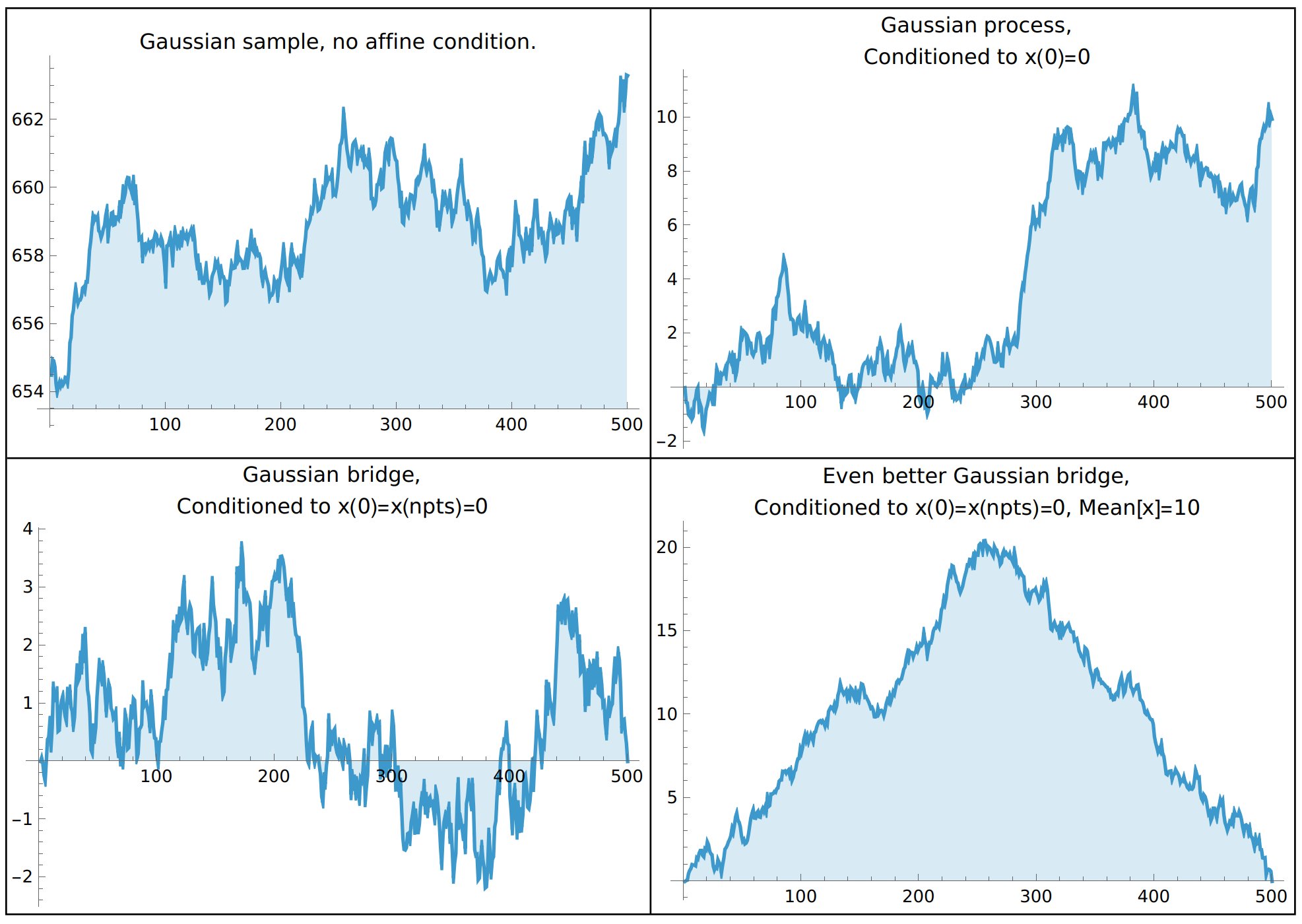
One-Dimensional Gaussian Field Examples

We have all of these fancy tools, and so I can’t help myself from throwing them all at the problem at once. Let’s allow for arbitrary linear constraints $Lx=b$ (allowing for both of these to be empty l=b={}). Our energy function will be the discrete second derivative with a mass term \(E=\sum_i (-x_i (x_{i+1}+x_{i-1}-2x_i)/\Delta x^2 + m^2 x_i^2),\) and we’ll build in free boundary conditions. If we want to fix boundary conditions, then we’re forced to do that through conditioning! At the end of the day I’m pretty satisfied with the images, especially with “Gaussian mt. Everest.”

(*
Random sample of a 1D scalar field with energy function (aka x.\
Hessian.x aka x.precision matrix.x)
E=\sum_i K (-x_i (x_{i+1}+x_{i-1}-2x_i)+m^2 x_i^2),
subject to linear constraints l.x==b. \
Free boundary conditions are assumed, \
so we need m>0 for the problem to be well-defined.
 *)
gaussianField1D[npts_, m_, k_, l_ : {}, b_ : {}] := 
  Module[{cov, hessian, sample, dist},
   (* Construct the hessian desired. 
   The rules specified first take precedence, 
   then we specify the diagonal bands. *)
   hessian = SparseArray[
     { {1, 1} -> m^2 + k,
      {npts, npts} -> m^2 + k,
      Band[{1, 1}] -> m^2 + 2 k,
      Band[{1, 2}] -> -k,
      Band[{2, 1}] -> -k}, {npts, npts}
     ];
   cov = Inverse[hessian];
   sample = RandomVariate[MultinormalDistribution[cov]];
   Which[
    (* case 1, no conditions *)
    Length[l] == 0, sample,
    (* case 2, one affine condition *)
    Dimensions[l] == {npts}, 
    sample + cov . l /(l . cov . l) (b - l . sample),
    (* case 3, multiple affine conditions *)
    Length[Dimensions[l]] == 2,
    sample + 
     cov . Transpose[l] . 
      Inverse[l . cov . Transpose[l]] . (b - l . sample)
    ]
   ];
npts = 500;
myplot[vector_, label_] := 
  ListLinePlot[vector, PlotLabel -> Style[label, Black], 
   ImageSize -> Medium, Filling -> Axis];
plot1 = myplot[gaussianField1D[npts, 0.0001, 10], 
   "Gaussian sample, no affine condition."];
plot2 = myplot[gaussianField1D[npts, 0.0001, 10,
    Table[If[i == 1, 1, 0], {i, 1, npts}],
    0
    ], "Gaussian process,\nConditioned to x(0)=0"];
plot3 = myplot[gaussianField1D[npts, 0.0001, 10,
    {Table[If[i == 1, 1, 0], {i, 1, npts}],
     Table[If[i == npts, 1, 0], {i, 1, npts}]},
    {0, 0}
    ], "Gaussian bridge,\nConditioned to x(0)=x(npts)=0"];
plot4 = myplot[gaussianField1D[npts, 0.0001, 10,
    {Table[If[i == 1, 1, 0], {i, 1, npts}],
     Table[If[i == npts, 1, 0], {i, 1, npts}],
     Table[1/npts, {i, 1, npts}]},
    {0, 0, 10}
    ], "Even better Gaussian bridge,\nConditioned to x(0)=x(npts)=0, \
Mean[x]=10"];
Grid[{ {plot1, plot2}, {plot3, plot4} }, Frame -> All]

If we were taking many samples, inverting the Hessian is defensible. But if we take a single sample there’s a better way to do things, where we never find the covariance matrix explicitly:

gaussianField1Dfaster[npts_, m_, k_, l_ : {}, b_ : {}] := 
  Module[{hessian, sample, dist, choleskyU, solver, uu},
   (* Construct the hessian desired. 
   The rules specified first take precedence, 
   then we specify the diagonal bands. *)
   hessian = SparseArray[
     { {1, 1} -> m^2 + k,
      {npts, npts} -> m^2 + k,
      Band[{1, 1}] -> m^2 + 2 k,
      Band[{1, 2}] -> -k,
      Band[{2, 1}] -> -k}, {npts, npts}
     ];
   
   
   choleskyU = CholeskyDecomposition[hessian];
   solver = LinearSolve[choleskyU];
   sample = solver[RandomVariate[NormalDistribution[], npts]];
   Which[
    (* case 1, no conditions *)
    Length[l] == 0, sample,
    (* case 2, one affine condition *)
    Dimensions[l] == {npts}, 
    uu = LinearSolve[hessian, l];  
    sample + uu/(l . uu) (b - l . sample),
    (* case 3, multiple affine conditions *)
    Length[Dimensions[l]] == 2,
    uu = LinearSolve[hessian, Transpose[l]];
    sample + uu . Inverse[l . uu] . (b - l . sample)
    ]
   ];

Appendix: Extra derivations and Practice Problems

Schur Complements

Question: Given a matrix which can be decomposed into block matrices $M=\begin{bmatrix}A & B\ C & D\end{bmatrix},$ find the block-wise entries of $M^{-1}.$ Organize your answer such that the matrix $M/D=A-B D^{-1}C$ is used. What is $M/D$ called? (Assume everything that needs to be invertible is invertible).

Hint: $M/D$ is called the Schur complement of $D$ in $M.$ Start by doing blockwise Gaussian elimination (if you choose a different order of elimination you’ll get $M/A$ instead of $M/D$) to get an LDU decomposition of $M$, which can be easily inverted and expanded.

Answer: For Gaussian elimination, to get a block diagonal matrix first hit $\begin{bmatrix}A&B\ C&D\end{bmatrix}$ with $\begin{bmatrix}I&0\ -D^{-1}C&I\end{bmatrix}$ from the right and $\begin{bmatrix}I&-BD^{-1}\ 0&I\end{bmatrix}$ from the left. This gives…

Question: Prove the Woodbury identity. That is, given matrices of commensurate dimension and given that the inverses exist where needed, show:

Hint: For $M=\begin{bmatrix}A&B\ C &D\end{bmatrix},$ look at the two ways of writing the block entries of $M^{-1}$ in terms of the Schur complements $M/D =A-B D^{-1}C$ and $M/A=D-C A^{-1}B.$

Answer: Consider the matrix $M=\begin{bmatrix}A & B\ C & D\end{bmatrix}.$ The formula for the Schur complement $M/D =A-B D^{-1}C$ gives

The top left entry gives the identity

To match with the form usually given, replace $D\mapsto -D^{-1}.$

Question: Consider the project of conditioning a multivariate Gaussian on a set of linear constraints $Lx=b$ by imposing a quadratic penalty

Take the limit as $\kappa\to\infty$ to find the conditioned covariance matrix and new mean. Assume $LL^T$ is invertible.

Hint: The new Hessian is $A_\kappa=A+\kappa L^TL$ and new source term $h_\kappa=A\mu+\kappa L^Tb.$ From this we know the new mean and new covariance matrix. Apply the Woodbury identity:

Answer: Expanding in the exponent gives:

The Woodbury identity gives:

The mean is $\Sigma’ h’,$ giving:

This limit always gives me trouble. $(A\kappa^{-1}+L^TL)^{-1}$ is singular as $\kappa\to \infty$ but acting on $L^T$ projects this singular part out. We can first apply Woodbury, then factor things out and get a miraculous cancellation:

Therefore:

Fresnel Integral Derivation

Question: Calculate the Fresnel integral $\int_{-\infty}^\infty \exp\left(\pm i a\frac12 x^2\right)\mathrm{d}x$ where $a\gt 0.$

Hint: Shift contours to the real line, you’ll have to choose a different contour for each sign. If you want to be rigorous about bounding the contours, the identity $\sin\theta \ge 2\theta/\pi$ for $0\le \theta \le \pi/2$ comes in handy.

Answer: The result is

or if $a$ is allowed to have a sign,

To outline the proof (for $a\gt 0$), consider the “+” sign. Take a contour from $x=0$ to $x=R,$ then along the arc from $x=R$ to $x=e^{i\theta}R,$ then in a straight line to the origin. Cauchy’s theorem gives:

For the “+” sign in the exponent, if we take $\theta=\pi/4$ then the third integral is just the Gaussian integral $\int \exp(-ay^2/2)\mathrm{d}y$ times a phase. So it remains to bound the middle term as $R$ goes to infinity. We find (using the hint $\sin\theta \ge 2\theta/\pi$):

This vanishes as $R\to\infty,$ therefore

Question: Calculate the improper oscillatory integral $Z=\int \mathrm{d}^d x\exp(\frac{i}{2} x^T A x+i J^T x)$ where $A$ is positive definite. What about when $A$ can have zero or negative eigenvalues?

Hint: Recall the integral

Another common approach is to use the “$i-\varepsilon$ prescription” (for the positive definite case).

Answer: We have, for positive definite $A,$

We’ll prove the general case. Imagine doing an orthonormal $PDP^{-1}$ decomposition of $A.$ For each zero mode, we get a factor of $2\pi\delta(\tilde{J}_i).$ The positive and negative modes give a factor each:

Once we transform back into the original basis, we find our integral:

where $\det’ |A|$ means we take the product of the absolute values of the nonzero eigenvalues, $K=\ker A,$ $k=\dim K,$ $A^+$ is the Moore-Penrose pseudoinverse (which has eigenvalues $1/\lambda_i$ for every nonzero eigenvalue of $A$, and $0$ for every zero eigenvalue of $A$), and $J$ has been decomposed into $J_K\in\ker A$ and $J_\perp.$ Note that since $A^+$ naturally zeroes out everything in $\ker A,$ we don’t really need to write $J_\perp$ and can just write $J^T A^+ J.$